Hello everyone,
Today, I will discuss ancestry analysis. In this context, I will use the term “admixed” to refer to individuals whose genetic makeup is composed of two or more parental populations, and “non-admixed” to describe individuals whose genetic material comes from a single parental population. I want to clarify this distinction because, if we trace our ancestry far enough back in time, we realize that no one is really non-admixed. Let’s say that human populations are quite enthusiastic about sharing genetic information ( ͡° ͜ʖ ͡°).
When we talk about ancestry inference, we can do it in three different levels: (i) populational, (ii) individual and (iii) local or chromosomal ancestry.
Disclaimer: In this post I will discuss a little about methods that I use. Some of them are old/cringe.
Populational ancestry
The population ancestry you infer reveals the contribution of each parental population to the genetic makeup of your entire population. Alternatively, when using clustering analysis, it shows where your population stands in comparison to the parental populations.
Methods: Principal Component Analysis (PCA) and ADMIXTURE.
For both methods you want use QCed data (Genetic QC Post) and independent variants (aka remove Linkage Disequilibrium).
Principal Component Analysis (PCA)
PCA is a dimensionality reduction technique that transforms data into principal components representing the variation within the dataset. PCA is data-driven, meaning the results are solely based on the input data. There are several ways to perform PCA:
- PCA without reference: The PCA reflects the genetic variability within your dataset. This result may reflect genetic variation not associated with ancestry.
- PCA with parental populations: In this approach, you include parental populations in your dataset, and the genetic differences between these populations may help guide the components. However, this is not always guaranteed, especially if the sample size of your reference population is smaller than that of your target data.
- Projected PCA: Here, you perform PCA using only the reference population and then project your target samples onto the reference population’s principal components. In this analysis your PC will only reflect the genetic variation present in the reference data
It is important that, in both 2 and 3, your reference and target data have the same SNPs
Figure 1: Projected PCA for a very diverse cohort

ADMIXTURE-like methods
ADMIXTURE (or STRUCTURE, or the newer version known as Neural ADMIXTURE) is a software tool used for maximum likelihood estimation of individual ancestries from multilocus SNP genotype datasets (as defined in [1]). In simpler terms, ADMIXTURE is a clustering algorithm that attempts to group samples based on genetic similarities.
You can run ADMIXTURE in two modes: unsupervised and supervised. In unsupervised mode, ADMIXTURE uses the dataset itself to build clusters based on genetic similarities. In supervised mode, you provide a reference dataset, and the method assumes these samples are non-admixed, using them to guide the clustering process.
An important note: avoid statements like “sample X is Y% European.” Since ADMIXTURE is a clustering algorithm, not a classification tool, it’s more accurate to say “sample X is Y% similar to the European reference dataset.”
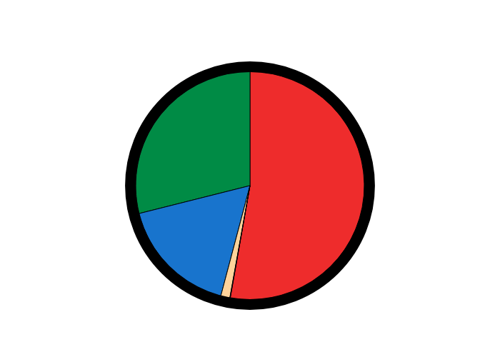
Figure 2: A pie chart built using supervised admixture for a population
Individual ancestry
When performing individual ancestry analysis, the goal is to determine the parental contributions to the genetic makeup of a single individual. You can use the same methods as in population ancestry analysis, but instead of focusing on population-level data, you will analyze the genetic information of an individual.

Figure 3: Artistic plots for individual ancestry analysis. The three plots have the same proportions and it is random numbers. You can always play safe and use pie charts.
Local or chromosomal ancestry
Individual ancestry analysis can be very useful, but it lacks precision. In my last ancestry test (performed using Ancestry Informative Markers in 2013), the results indicated that my genetic makeup was 50% similar to European, 27% African, and 23% Native American. While these percentages are interesting, they don’t guarantee that these proportions are evenly distributed across my entire genome. In fact, it’s expected that some regions of my genome may be more European than others, due to the way recombination occurs.
In this gif we can see how the admixture events can create smaller ancestry fragments with more generation.

Figure 4: Gif with an example how recombination can create fragments of ancestry
By using high-density variant arrays or Whole Genome Sequencing (WGS) data, we can infer the ancestry for specific regions of each chromosome in an individual. This is particularly useful because local ancestry — the identification of specific ancestral contributions to different parts of the genome — can improve genotype-phenotype association studies in admixed populations. These populations are often underpowered in traditional studies due to their genetic heterogeneity.

Figure 5: On the left, an individual with more than 90% European (EUR) ancestry shows the GBA gene inferred as Native American (NAT) and African (AFR), represented by the green and blue triangles. On the right, an individual with more than 90% Native American (NAT) ancestry shows the GBA gene inferred as European (EUR) and African (AFR), represented by the red and blue triangles. We selected the GBA gene because a recent study identified an African ancestry-specific risk locus in this gene [2].
To perform local ancestry analysis, you should begin with a quality-controlled (QCed) dataset for both the target (admixed samples) and the reference population. After identifying the common variants between the two datasets, you should phase both datasets in a way that ensures they share the same phase. Following this, you can infer the local ancestry and create plots. In Figure 5, we QCed our data using the LARGE-PD QC pipeline, obtained the list of common variants using an in-house script, phased both the target and reference datasets using the TOPMed Imputation Server, inferred the local ancestry with G-Nomix, and generated the plot using Tagore.
Methods: RFMix v1 (I don’t like RFMix v2), LAMP-LD, G-Nomix (I am actually using this one)
I think that is a good introduction about the ancestry analysis and a good start for the people that wants to study more about it. There are other methods (that I do not have experience) to perform analysis based on ancestry, but this method are focused in studying population demography (example Chromopainter, fineSTRUCTURE, Hallental Methods, etc). If you have questions (philosophical or methodological) put on the comments.
Special thanks to @paularp and @psaffie that participated in some analysis described in this post.
References
[1] Website of ADMIXTURE
[2] Rizig, M., Bandres-Ciga, S., Makarious, M. B., Ojo, O. O., Crea, P. W., Abiodun, O. V., Levine, K. S., Abubakar, S. A., Achoru, C. O., Vitale, D., Adeniji, O. A., Agabi, O. P., Koretsky, M. J., Agulanna, U., Hall, D. A., Akinyemi, R. O., Xie, T., Ali, M. W., Shamim, E. A., . . . Fang, Z. (2023). Identification of genetic risk loci and causal insights associated with Parkinson’s disease in African and African admixed populations: a genome-wide association study. The Lancet Neurology , 22 (11), 1015–1025. Redirecting